It's not an overstatement to say that there has been "a lot" of literature written about industrial process control and the venerable PID control algorithm.  However, if there's been a lot written about the specific implementation of PID control for Turbomachinery Control applications, I couldn't find it. So, to fill a hole that may or may not exist, in the next couple of posts, we'll be informally discussing PID use for Turbomachinery Control (TMC) applications.

In this post, we'll start our discussion with the basics to standardize on a vocabulary.

In the next post we’ll talk about the variations to PIDs used for turbomachinery control (TMC) and where they are used,  We'll also talk about signal "filtering" as it relates to TMC.

In the final post of this series, we'll discuss some of the challenges in “tuning” turbomachinery controls, some tuning methods worth consideration (pros and cons) along with some simulation examples.

Turbomachinery PID Control (part one)

To begin with, in order to make sure we are using the same vocabulary, we need to work through some basic definitions, starting with process types. 

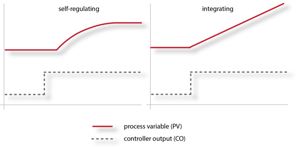
Industrial process types  are typically defined as either;  self-regulating, integrating, or “runaway.”

Self-Regulating processes: are processes that gradually "settle out" after a "step" change in the controller output. 

Integrating processes; are processes that continue to change at a steady state (mostly linear ramp) after a "step" change in the controller output.

Runaway processes; are unstable processes that have an uncontrolled (runaway) acceleration rate (e.g., exothermic chemical reaction). 

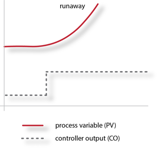
Most TMC related processes are self-regulating, a couple are integrating, and I can't think of any TMC related "runaway" types; so we'll leave the runaway process here.

More general process jargon - 

Process Gain - is the amount the process variable changes, for a given change in the controller output (CO).

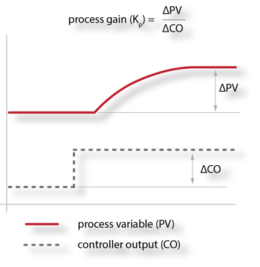
The change in CO is typically expressed as a percent (which is probably how you will find the controller output defined within the PLC, DCS, digital governor etc.). By convention the process gain is usually described as %/% (or unit-less) so the change in the process variable (PV) also needs to be expressed as a percent (you may need to convert it). 

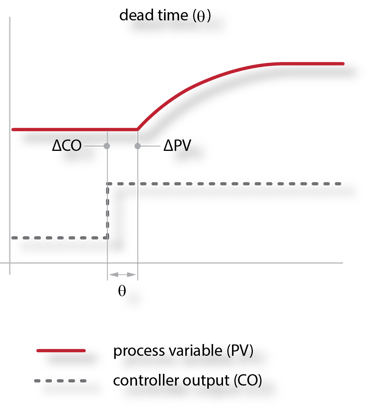
Dead Time: is the time it takes for the process variable to start changing after a change in the controller output. In the following cartoon the process dead-time is pretty easy to see. Unluckily, with many TMC loops, there's very little process dead-time and it can be devilishly hard to quantify. We'll talk more about this when we talk about tuning. 

Lag (time constant): is the time a process takes to reach it's new steady state after a change in the controller output. The lag time starts when the dead-time ends. Process loops with short time constants reach their "final value" quicker than process loops with longer time constants (all else being equal).

For many "open-loop" tuning rules, we are only concerned with the time it takes for a process to reach 62.3% of it's final value after a change in the controller output (more on this when we talk about open loop tuning techniques).

Integration rate (for integrating process): depending on who you talk to, the process gain for an integrating process can be calculated a couple of different ways (as a process gain (sets up for "Lambda Tuning") or an integrating rate. We like using integrating rate posited by Jacques Smuts in "Process Control for Practitioners", which looks a lot like process gain, except that it includes time in it's derivation. 

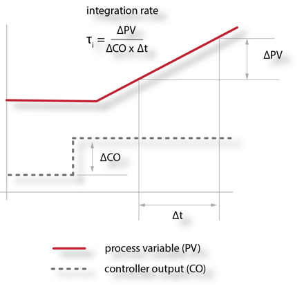
The previous cartoon depicts an integrating process that is integrating from steady state.

The integrating process could also be unsteady (continually integrating):

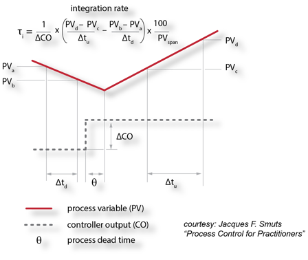
We'll get into the calculation of the integrating rate in more depth when we talk about tuning. 

........

That's about it for defining general process characteristics (at least for the time being). If we can describe the type, gain, dead time, and time constant for a given process, we are well on our way to being able to tune it. 

In this next part we'll define the  jargon we use when we are talking about turbomachinery PID controls.

A quick contextual note - tuning constants aside, the basic digital PID uses a setpoint (SP) and  a process variable (PV) to generate a controller output. 

Target: At Tri-Sen we typically use a setpoint target in conjunction with the controller setpoint. The target is where we want the setpoint to be. That is, if we wanted a steam turbine speed setpoint to be at 3456 rpm, we would enter a target of 3456 rpm through some sort of operator interface.

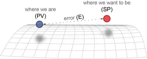
Setpoint (SP): The setpoint is what the PID uses for control, it's where we want the process to be. 

Here's how the whole target and setpoint thing works:

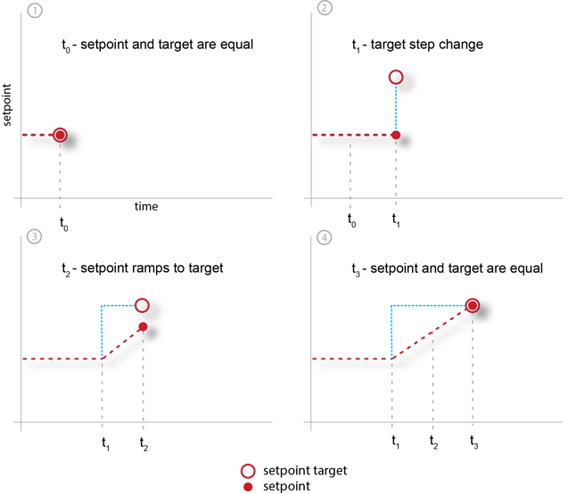
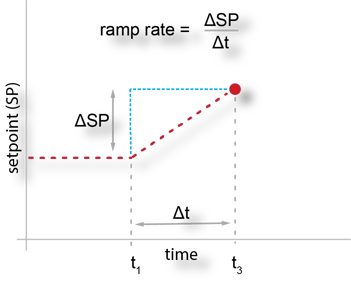
Ramp-Rate: The ramp-rate is the rate that the setpoint is "ramped" to the target (using a "ramp" function). We ramp the setpoint to the target so that we don't create a large, instantaneous error, and an accompanying PID controller output "bump," when we want to make a significant change in where we are operating.  For example,  let's say we wanted to increase the speed of our turbine from 3456 rpm to 4000 rpm. When we enter a target of 4000 rpm, the setpoint will ramp from 3456 rpm to 4000 rpm at the programmed ramp rate. Usually, this ramp rate is expressed in engineering units over time; for this case, we might use rpm/second, but it could be expressed any number of ways.

Process Variable (PV): The process variable, or measured variable, or simply measurement, is where we are (from a controls/process perspective). It's the "process feedback" to the PID controller. Typical PVs for TMC include: speed, flow, pressure, power, and level.

Error (E): The error, or process error, as calculated by the PID controller is the difference between where we want to be (SP) and where we are (PV). This error is what the PID is trying to correct.

"No matter where you go, there you are."

- Buckaroo Banzai

Next, lets take a look at the "big three" PID control algorithms described in most textbooks and papers, and then “discretize” the form we use most often in TMCs.

Big Three PID Control Forms:

Some abbreviations to get started:

• CO = the PID controller output 
• E = error between the setpoint and process variable. 
• K_c = controller gain
• T_i = integral time
• T_d = derivative time
  
  

Parallel PID form: In the parallel PID form, the proportional, integral, and derivative "modes" are independent of each other, which means there are actually three gain settings; proportional (K_p), integral (K_i), and derivative (K_d).

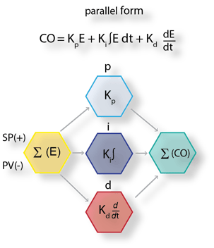
We don't really use this form for turbomachinery control (at least not at Tri-Sen). It's easy to understand but really hard to tune, so we'll leave it here. 

Interactive, series, classical, or real: According to Dr. Jacques Smuts, the interactive PID is based "on the way classical pneumatic and electronic PID controllers worked." For these controllers, there's an interaction between the integral and derivative terms.

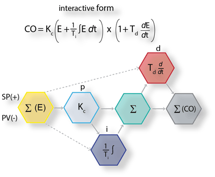
I'd say that we don't use it much at Tri-Sen but there's an interesting thing about the interactive form; if you aren't using the derivative action (a "PI"controller) - and we don't use derivative very often - it's the same as the non-interactive (our favorite) form - the one we'll talk about next.

Ideal, Standard, Non-interactive: the PID form we see a lot in TMCs.  It's called non-interactive because unlike the interactive form, there's no interaction between the derivative and integral terms. The big thing to remember here is that the controller gain (K_c) not only effects the "proportional' action, but it's also used by both the "integral" and "derivative" actions. 

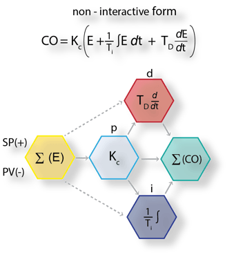
And, just as a reminder, if we don't use the derivative action, the interactive and non-interactive "PI" forms are the same.

"Discretizing" the non-interactive form: Before we go further, we need to “discretize” the standard (non-interactive) PID for use in a digital controller (go from analog to digital). Luckily, other people have already done the "mathmatical heavy lifting," which mostly includes approximations that take into account the controllers scan rate (as opposed to continuous time).

For the next couple of equations I'll be borrowing heavily from Liptak, "Instrument Engineers Handbook, 3rd Edition." He includes a "b" term in the calculations that we haven't included previously - it's just an offset (like a null position on an actuator control) and we won't worry about it too much. 

The discrete version of our non-interactive form -

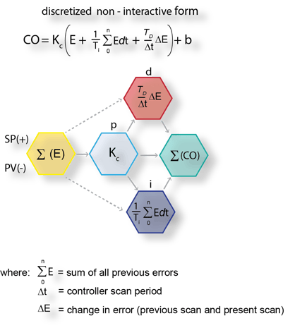
Up to this point, the PID controllers we have talked about are referred to as “positional” - the "entire" controller output  is recalculated each time the "error" is interpreted (every scan). The positional PID form is useful, but it's not the form we use as the basis for most of our controls. We need to go a little further and define a form called the "velocity" PID.

Velocity PID:  is the form we love so well, and the default control form for most of turbomachinery controls we deliver. We get to it by approximating the "derivative" of the positional form. 

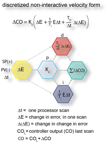
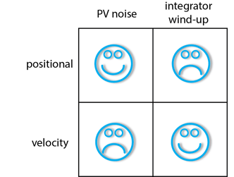
Positional vs. Velocity: the Positional PID tends to have better PV noise "immunity" than the velocity form because the gain term is acting on error and not the change in error (which could look like noise) . The downside of the Positional PID form is that the integral action can "wind-up" if the error is "sustained";  driving the controller output beyond 100% (hardware output physical limit) to the controllers mathematical limit (could be in the thousands). Unless there's external (from the PID) programming to limit the controllers integration, all of this excess "controller output" has to be "unwound" before the physical output comes off of it's limit.

We tend to use the velocity form for most TMC control loops and externally filter the process variable. 

A few more idiosyncratic definitions before we call it a day-

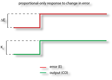
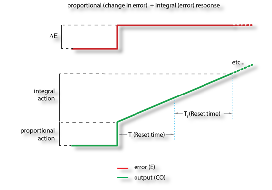
Proportional Term (P): The controller gain (K_c) is often referred to as the "proportional term." It's the primary controller setting for the interactive and non-interactive PID controllers. The proportional term (or controller gain) determines the controller's proportional response to a given error.

The "P" term for a PID is expressed as either:

• Controller gain (K_c)
• Proportional gain (K_p)
• Proportional Band (PB)

PB is the reciprocal of the controller gain, and typically it’s thought of as the percent change in the measured variable required to produce a 100 percent change in the output.

This means that the bigger the proportional band (or smaller the gain), the smaller the change in the controllers output for a given error.

Integral Term (I): Reset (also known as integral) is entered in seconds per repeat (and other times repeats per minute). It represents the time allotted to "repeat" the proportional action of the controller. As long as the error exists, integral action "repeats" the controller gain (proportional action) over each reset time. The bigger (longer) the reset time, the slower the controller response.

Derivative Term (D): Rate (also known as derivative) is entered in seconds. Derivative is often-times describe as a "feed-forward" - a point of contention for some. True "feed-forward" or not, the derivative allows the controller to "take predictive action" based on the rate of change (slope) of the error. Derivative adds the projected proportional contribution every "derivative" time period. As long as a rate of change in the error exists, the derivative action is applied (if it's enabled).

Increasing the derivative time can help to stabilize the controller response for some process loops, but too "high" of a derivative time, coupled with noisy process variables, usually causes the controller output to fluctuate too much, making for poor control.

Gain-on-error vs. Gain-on-measurement: It turns out that instead of using the change in error between the setpoint and the measurement to correct the output to the process (gain-on-error or GoE), we can use the difference (change) between the current and previous measurement values to correct the output (gain-on-measurement or GoM.) There are control loops ("quiet" integrating processes) where asserting the gain-on-measurement can be useful but your typical turbomachinery controller should be using gain-on-error.

Forward (Direct) vs. Reverse Acting: The action of the PID controller can be programmed so that if the process variable is greater than the setpoint, the output increases (valve opens) - this controller is said to be Forward (Direct) acting. An example of where you would use this type of action is with a level controller and the valve was at the bottom of the tank. If the level got too high (process variable > setpoint) then to prevent the tank from getting too full, the valve would open.

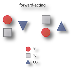
A reverse acting controller would close the valve if the process variable > setpoint. In our tank example it would be controlling the input of whatever was going into the tank directly, and close the control valve as the level increased above setpoint.

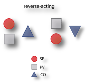
Speed control is typically reverse acting.

Cascaded Control: for many turbomachinery controls applications we "cascade" one PID control into another.  The general definition of a cascaded control can be a little wonky;

 ... a primary or master controller generates a control effort that serves as the setpoint for a secondary or slave controller. That controller in turn uses the actuator to apply its control effort directly to the secondary process. The secondary process then generates a secondary process variable that serves as the control effort for the primary process."

https://www.controleng.com/articles/fundamentals-of-cascade-control/

If you don't already know what cascaded control is,  a picture is probably worth 111 words: 

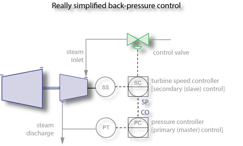
Let's say, for whatever reason,  our objective in the simplified example above is to control steam turbine back pressure. One way to accomplish this is by varying the turbine speed by "cascading" a pressure controller into the turbine speed control. The output of the pressure control PID is scaled as a speed setpoint to the turbine speed controller.

We'll talk more about cascaded control when we discuss PID controller tuning. 

And that's about it for this post. In the next post we'll talk about the application of turbomachinery control PIDs along with signal filtering. Be sure to let us know what you think about our blog - good, bad or indifferent (which is sort of bad).

Lastly, here's an additional controls related resource that we really like: 

https://blog.opticontrols.com/ a blog by Jacques Smuts PhD PE.

Thanks for your interest!